Example usage
To use QUICKLB it has to be imported first, if this fails please go to the Installation section.
import quicklb
Unbalanced reaction diffusion with QUICKLB
In this example we will create a reaction diffusion simulation which uses a loadbalancer for the chemistry calculation part (which is local), and a normal non-loadbalanced process for the diffusion process.
The easies and quickest way to get started is with the Loadbalancer object.
from quicklb import Loadbalancer
We have to create our domain, and work arrays and divide them over the number of processors, to reduce the amount of communication code necessary for the non-loadbalanced part we use shared-memory array (which are a bit more complex than normal numpy arrays). It also means that the example will only work if all processors have acces to the same memoryspace.
import numpy as np
from mpi4py import MPI
import matplotlib.pyplot as plt
import scipy.integrate
comm = MPI.COMM_WORLD

def allocate_shared_array(size):
  nbytes = np.prod(size) * MPI.DOUBLE.Get_size()
  if comm.Get_rank() != 0:
    nbytes = 0
  win = MPI.Win.Allocate_shared(nbytes, MPI.DOUBLE.Get_size(),comm=comm)
  buf, _ = win.Shared_query(0)
  return np.ndarray(size,dtype=np.float64,buffer=buf), win

# Using shared array we cheat a bit to  make it simpler
size = 30
A, winA = allocate_shared_array((size,size))
B, winB = allocate_shared_array((size,size))

# Calculate which part of the shared array is "local" to this processor
remainder = size%comm.Get_size()
slice_size = size//comm.Get_size()
start = int(slice_size*comm.Get_rank() + min(comm.Get_rank(), remainder))
end   = int(slice_size*(comm.Get_rank() + 1) + min(comm.Get_rank()+1, remainder))

A_local = A[start:end,:]
This gives us a slice on each processor which we fill up with an initial condition:
if comm.Get_rank() == 0:
  A[:,:] = 1.
  B[:,:] = 0.
  A[size//2-3:size//2+3,size//2-10:size//2+10] = 0.50
Secondly we need a structure to encapsulate these points such that the loadbalancer knows which data to communicate, how to encapsulate, and how to compute an interation
class Cell():

  def __init__(self,AA=None,BB=None):
    self.A = np.array([float('nan')],dtype=np.float64)
    self.B = np.array([float('nan')],dtype=np.float64)
    if AA != None:
      self.A = AA
    if BB != None:
      self.B = BB

  def compute(self):
    a = self.A[0]
    b = self.B[0]
    soln =scipy.integrate.solve_ivp(Cell.deriv,(0,1),(a,b),
        method='BDF', rtol=0.0001)
    self.A[0] = soln.y[0][-1]
    self.B[0] = soln.y[1][-1]

  def deriv(t,y):
    a, b = y
    abb = a*b*b
    adot =  - abb + 0.0545 * ( 1 - a )
    bdot =  + abb - ( 0.0545 + 0.062 ) * b
    return adot, bdot

  def serialize(self):
    return np.concatenate( (self.A.view(dtype=np.byte),
                            self.B.view(dtype=np.byte)))

  def deserialize(self, buffer):
    self.A[0] = buffer[0:8].view(dtype=np.float64)
    self.B[0] = buffer[8:16].view(dtype=np.float64)
This Cell class can either point to data when local, or store data when offloaded, furthermore a compute function is provided
We must create a list of cells that we want loadbalanced
cells = [Cell(A_local[i,j:j+1], B_local[i,j:j+1])
         for j in range(size) for i in range(A_local.shape[0])]
Then we can create the Loadbalancer:
lb = Loadbalancer(cells, "SORT", 0.01, 0.01, 3)
As an intermezzo we also need a diffusion operator which is separate from the loadbalancer:
A_diff = np.empty(shape=(A_local.shape[0]+2,A_local.shape[1]+2))
B_diff = np.empty(shape=(B_local.shape[0]+2,B_local.shape[1]+2))
def diffuse():
  # Perform diffusion over the local field + boundaries (this is where we cheat with shared memory arrays
  A_diff[1:-1,1:-1] = A_local
  # local periodic boundaries
  A_diff[0,1:-1] = A[start-1,:]
  A_diff[-1,1:-1] =A[end%A.shape[0],:]
  # "communicate" boundaries,
  A_diff[1:-1,0] = A_local[:,-1]
  A_diff[1:-1,-1] =A_local[:,0]

  B_diff[1:-1,1:-1] = B_local
  # local periodic boundaries
  B_diff[0,1:-1] = B[start-1,:]
  B_diff[-1,1:-1] =B[end%B.shape[0],:]
  # "communicate" boundaries,
  B_diff[1:-1,0] = B_local[:,-1]
  B_diff[1:-1,-1] =B_local[:,0]

  LA       =                       A_diff[ :-2, 1:-1] + \
             A_diff[1:-1, :-2] - 4*A_diff[1:-1, 1:-1] + A_diff[1:-1, 2:] + \
                               +   A_diff[2:  , 1:-1]
  LB       =                       B_diff[ :-2, 1:-1] + \
             B_diff[1:-1, :-2] - 4*B_diff[1:-1, 1:-1] + B_diff[1:-1, 2:] + \
                               +   B_diff[2:  , 1:-1]
  return LA,LB
And with this loadbalancer + diffusion operator we can iterate to our heart’s content:
number_of_iterations = 100
lb.partition()
for i in range(number_of_iterations):
  winA.Sync()
  winB.Sync()
  comm.Barrier()
  LA,LB = diffuse()

  # Chemistry
  if i%10 == 1:
    lb.partition()
    lb.partitioning_info()
  if i%10 == 0:
    if comm.Get_rank() == 0:
      plt.imshow(B)
      plt.show(block=False)
      plt.pause(0.03)
  lb.iterate()

  A_local[:,:] = A_local + 0.1*LA
  B_local[:,:] = B_local + 0.05*LB
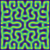
Lastly we can create visualise this quite easily with matplotlib!
winB.Sync()
comm.Barrier()
if comm.Get_rank() == 0:
  plt.imsave("gray_scott_rd.png",B)
  plt.show()
Timings |
Normal |
Load Balanced |
|---|---|---|
2 MPI procs |
50.31 s |
51.63 s |
3 MPI procs |
46.02 s |
41.25 s |
4 MPI procs |
39.54 s |
33.04 s |